| Slide rules HOME page | INSTRUCTIONS | A-to-Z |
Basics of slide rule use
Parts of a rule, logarithms, linear v logarithmic scales, naming the scales, reading the scales, gauge points
A slide rule consists of three basic part: the main body of the rule, known as the stock (or stator or body), the movable part, known as the slide, and a moveable cursor (or indicator) made of clear glass or plastic.
On the stock and slide there are marked a number of scales. In the simplest slide rules there may be two scales on the stock and two on the slide. On a complex rule there may be a total of twenty or more scales. Some rules have scales on one face only and a cursor which can only be used on that face; these are referred to as "simplex" rules. Others have scales on both faces with a cursor which can also be used on both faces; these are referred to as "duplex." A very common intermediary between the two forms is found on rules with scales only on one face of the stock but on both sides of the slide. Within this latter group there are two variants; usually a small mark on the back of the stock allows the slide to be used without removing it but some times the slide has to be removed and inserted with its face reversed.
Sometimes the stock has standard measuring rulers, marked in inches or centimetres. These perform no role in calculation.
The graduations on the scales are so arranged that by alignment of scales on the stock and slide it is possible to perform mathematical calculations. Some slide rules have additional marks on the scales. These are known as gauge points and are used to facilitate certain types of calculation and their use is described in a separate chapter.
The main purpose of the cursor is to enable the the correct alignment of different parts of the slide rule which are not immediately adjacent. For this purpose a cursor has a central hairline, a fine line engraved on or set into the cursor. On duplex rules the cursor will also allow the alignment of scales on both faces of the rule. On some rules the cursor extends over the edges of the rules allowing scale to be placed there.
The cursor may be of glass or plastic. In the case of glass cursors, the cursor is set into a metal frame. The cursor has a small spring which fits into the grove of the stock and, whilst allowing the cursor to slide, helps to hold it in place.
In addition to the central hair-line, a cursor may have other hair-lines designed to facilitate frequently performed types of calculations. This type of cursor is more common on European rules than on ones from the USA.
Slide rules are based on the concept of logarithms. Although a knowledge of logarithms it is not necessary to be able to use a slide rule, it does help you to understand what you are doing.
If you multiply a number raised to two different powers, the result is equal to the same number raised to the sum of the powers.
A very simple case would be:
22 x 23
= 2(2+3) = 25
That is:
4 x 8 =
32
Another, slightly more general, example might be:
10a x 10b =
10(a+b)
This suggests a way in which multiplication, difficult with complicated numbers, can be replaced by addition, much easier even with complicated numbers. If "a" is chosen so that 10a equals the first number to be multiplied and "b" so that 10b equals the second number to be multiplied then all that is needed is a way to work back and find out the number equal to 10(a+b). If, say, one wanted to multiply 2 and 3 then "a" would have the value of 0.301 (since 100.301 equals 2) and "b" would have the value 0.477 (since 100.477 equals 3). The value of 0.301 in known as the logarithm of 2 and the value of 0.477 as the logarithm of 3. The result of the multiplication is 100.778 (that is 10(0.301+0.477) ) which in turn is equal to 6. The value 6 is known as the antilogarithm of 0.788. Incidentally, the above example uses 10 raised to different powers; other numbers could be used as the base but 10 was the most common.
A similar procedure can be used for division, except that the powers are subtracted.
A slide rule gets round this complication by making the distances on the scales proportional to the logarithms of the numbers marked on the scales. By positioning two scales, one on the slide and one on the stock, in such a way that you are adding the distance of one scale to another, you are effectively adding the logarithms of these numbers and therefore multiplying them. Similarly, by positioning the scales to get the difference in distance between two numbers, you are effectively dividing them.
Slide rules also make use of another feature of logarithms. Any number can be represented by another number between 1 and 10 multiplied by ten raised to a power. For example 761 is equal to 7.61 times 100 (i.e. 102); 0.325 is equal to 3.25 times 0.1 (i.e. 10-1). The principal scales of slide rules have numbers from 1 to 10 only.
Linear versus logarithmic scales
Most measuring rules have linear scales. That is, the graduations are divided evenly. With such a rule it is so obvious to say, for example, that the distance between the marking for 2 and 4 is the same as the distance between 6 and 8, that it is rarely said.
With scales graduated logarithmically the ratio between numbers is always represented by a constant distance. Take a look at the D scales of a typical slide rule. The total length of the scale will usually be close to 250 mm. The distance between the 1 and the 2, between the 2 and 4, between the 4 and 8 and between the 3 and 6 (in each case the second number of the pair is twice the first) will be identical (around 75 mm).
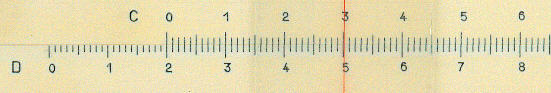
Although it is not normally done, it is possible to use a pair of linear scales for addition. The picture below, from a German learner's rule, does show just that. The zero of the C scale is against the 2 of the D scale and the cursor hair line, on the 3 of the C scale, shows the total of 2 plus 3 equal to 5. What are saying is, quite simply, that 2 centimetres plus 3 centimetres is 5 centimetres. What is more, every mark on the D scale is equal to the value of the C scale plus 2. Not exactly rocket science!
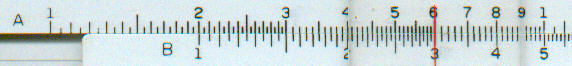
The next diagram show the equivalent for logarithmic scales. In this case the 1 of the B scale is against the 2 of the A scale and cursor hairline (red), on the 3 of the B scale, shows the 2 times 3 equals 6. Also, whereas with the linear scale the setting showed a constant addition, this shows a constant multiplication by 2 since every number of the A scale is twice the value on the B scale. You will have noticed that 1.0 for multiplication on the logarithmic scale replaces 0.0 for addition on the lniear scale; in effect both adding 0.0 to a number and multiplying a number by 1.0 leave the value unchanged. (As you may also have noticed, and this is a feature of many slide rules, the scales on this slide rule restart at 1 rather than moving on to 10. ). What we have done is very similar to what we did above but since we are adding distances representing the logarithms of number, rather than the numbers themselves, we have ended up multiplying numbers rather adding them. Again not exactly rocket science but very ingenious.
Most scales on most rules have a letter or other symbols to identify them. Even the simplest rule usually has four scales labelled A, B, C and D. The C scale, on the slide, and the D scale, on the stock, are used for most calculations involving multiplication and division and cover one logarithmic cycle; that is they have the numbers from 1 to 10. The A scale, on the stock, and the B scale, on the slide, cover two logarithmic cycles, that is they have the numbers from 1 to 10 and 10 to 100, and represent the square of the numbers on the D and C scales.
Among the other scales you will find are:
In the A-to-Z we describe the use of these and other scales. Over the years the naming of these scales became more or less standardised. If you have a rule and cannot identify the scales have a look at the section on scales.
As you may have gathered from the above, the uneven separation between the graduations means reading values is not straightforward.
The image below (left bigger than the screen to maintain the detail) shows typical scales from two different slide rules. Both scales cover the range 1 to 10 but are marked differently. In the lower image, the graduations between 1 and 2 are marked 1.1 to 1.9, in the upper image they are marked 1 to 9. Although at first the lower arrangement might seem more sensible, with a little practice either arrangement will become familiar. You might also find other variations, for example some rules mark the graduation for 2.5.
One concept a user needs to be familiar with is that of "significant figures". The number for p (the ratio of the circumference to the diameter of a circle) can be expressed as 3.141592654 to 10 significant figures; that is the number is given with 10 separate digits. If it was given as 3.14, it would be represented as having 3 significant figures. On a slide rule you can normally work to a precision of 3, and sometimes 4, significant figures.
The lettering and lines in red show pairs of values on the two types of rule. The first number (1.142) shows that at the left hand end of a rule it is usually possible to estimate a value to a precision of a 4 significant figures. Though in this example (where the red line is thicker than the marking) it would be difficult to decide whether the value was 1.142 or 1.141. As we move along the rule to the next number (2.05) we already see that three significant figures are all the we can read with accuracy. The next number is included to show a reading where the value corresponds to one of the marked graduations. Another difference between the rules is demonstrated by the number 4.36, which in the upper scale corresponds to a marked graduation but in the lower scale has to be estimated. As we move further to the right was see that the space between graduations becomes smaller and more and more care is needed in the estimation of the number.
It would be a good idea to look at all the figures in red and make sure the numbers and graduations make sense to you.

Now you should make a note of what you think is the value of each of the lines marked in green. The answers are given here. Do not worry too much if your estimate of the final figure is different by 1.
Two final points. Firstly, logarithmic scales are cyclical. A single cycle goes from 1 to 10; a double cycle goes from 1 to 100. The above diagrams show a single logarithmic cycle. Secondly, because the scales are cyclical the number 10 is sometimes not marked but the cycle is assumed to begin again from 1. The lower of the two scales above has a 10 at the right hand end, the other has a 1.
Other scales, for example those related to trigonometrical functions, are not the same as those above, but with a bit of practice they will be as easy to read.
On both of the above scales there is a p marked with a short line at 3.14; this is ratio of the circumference of a circle to its diameter. The upper scale also has a C marked at 1.13; this is equal to Ö (4/p) and is also used calculation involving circles. These marks represent frequently used constant values and are called gauge points. For more details look at the section on gauge points.